
Understanding WindESCo's EIA Methodology in a little more detail
Overview:
In an environment of skepticism, we bridge the gap between the AEP improvements our wind operators expect, and the service agreements signed with their OEMs. We look at high resolution data, through proprietary algorithms to find anomalies, fix them, measure them and deliver AEP performance gains. Our independent measurement methodology targets improving the revenue position of our customers, pays for itself within 12 months, and will return up to seven times the investment.
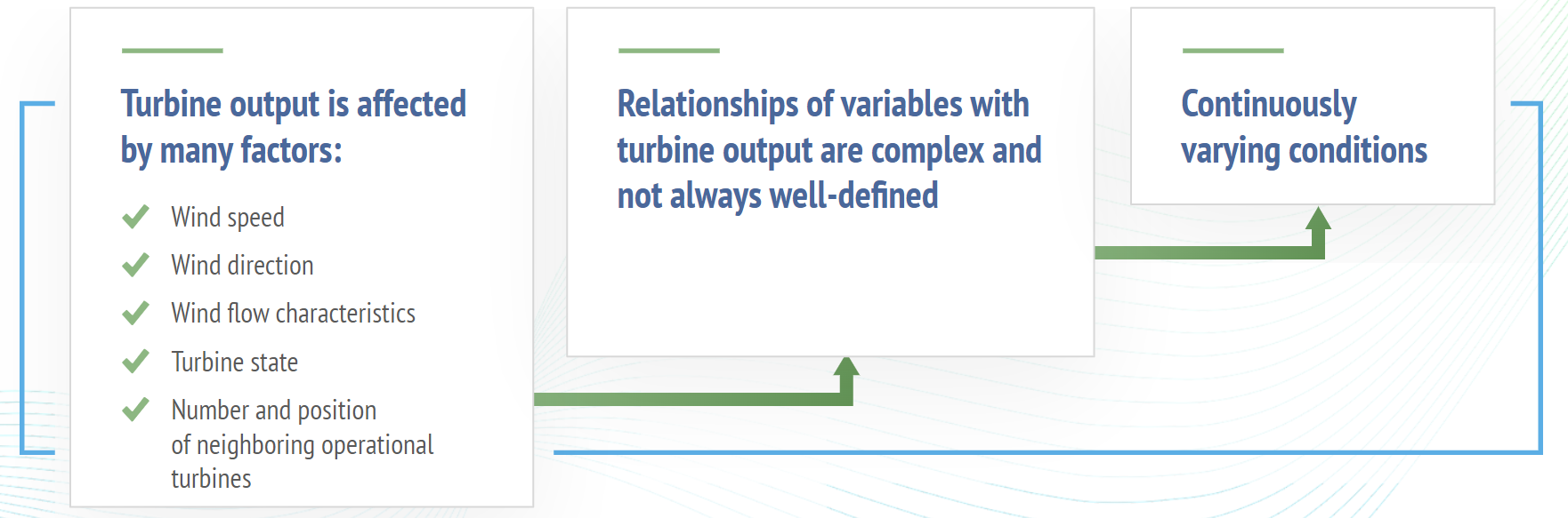
Challenges of Measurement:
Wind is complex, which makes changes in output difficult to measure
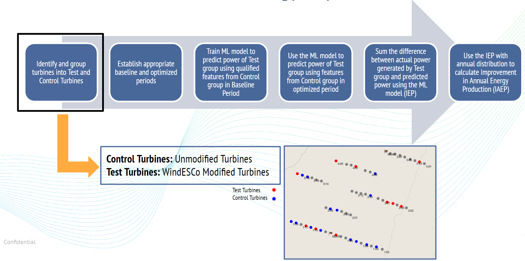
The WindESCo Method for Energy Improvement Assessment:
Step 1: A selection of control (unmodified) and test (corrected) turbines is made
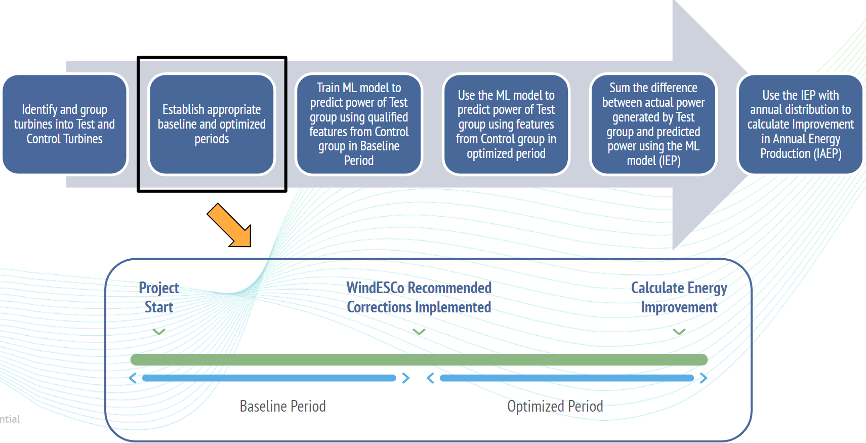
Step 2: The period over which the EIA will be conducted (~90 days is required) before and after the change
Step 3: The machine learning (ML) model is trained and used to determine the change in power
Note:
- The control turbines are given a similarity score before / after the change to the test turbines to confirm the two time periods are a valid
- A high similarity score means that the two time periods have similar data statistics and distributions, so a comparison between the two periods is valid
- A low similarity score means that the two time periods are too dissimilar, and a comparison is not valid
- The energy comparison tool has recently been improved for robustness, data filtering and control turbine evaluation.
- IEP uncertainty comes directly from quantile regression
- IAEP uncertainty: delta power vs actual power, scatter plot of points with their own uncertainty. Combine using Monte Carlo simulations
Summary:
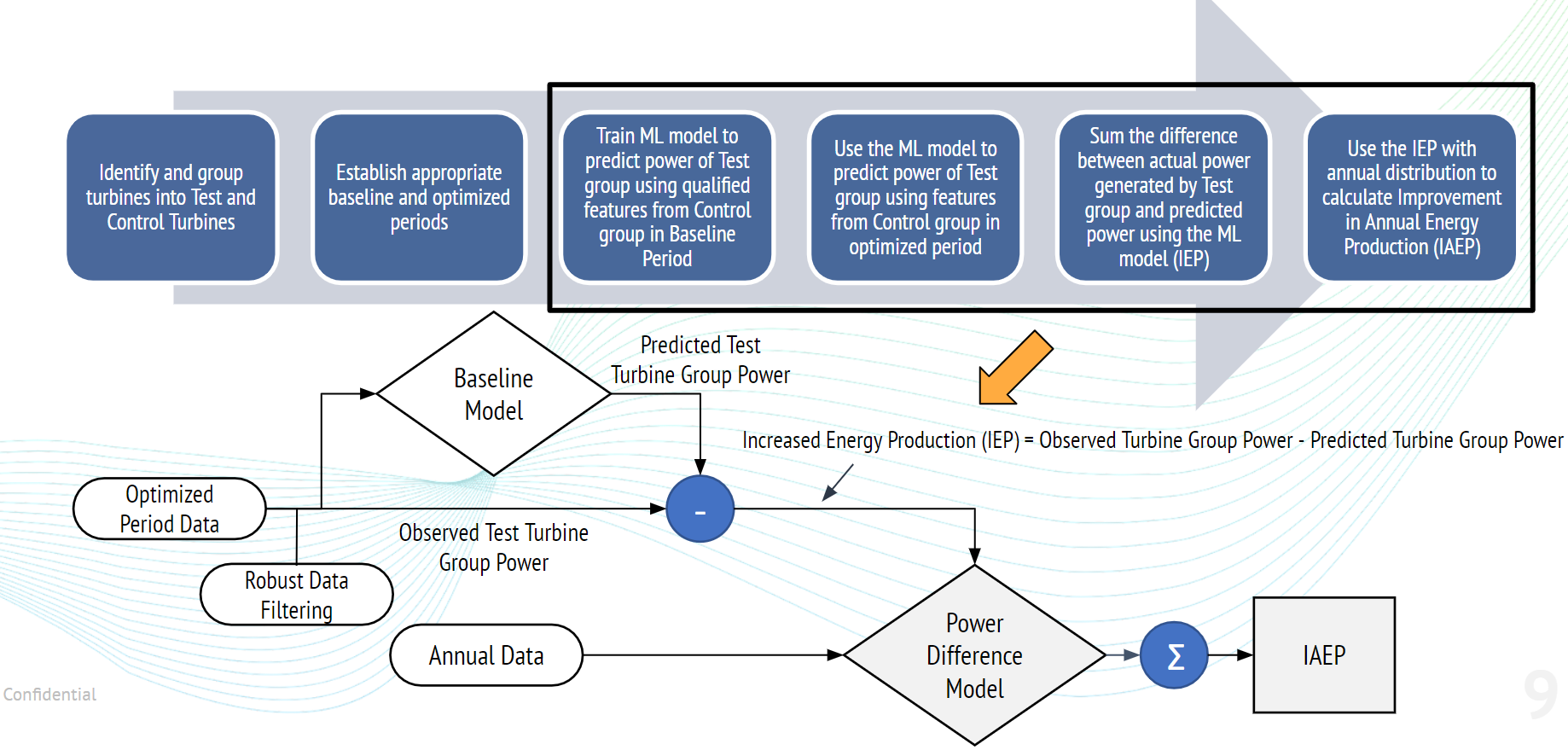
The Increase in Annual Energy Production (IAEP) is calculated in four steps:
- Predict power in optimized period using the ML model trained to the baseline period
- At each time step in the optimized, subtract the predicted power from the measured power
- Train a model to predict the power difference calculated above
- Use annual wind data to generate an annual energy improvement based on this power difference model
The IAEP estimate is accurate with an uncertainty of +/- 0.3%.
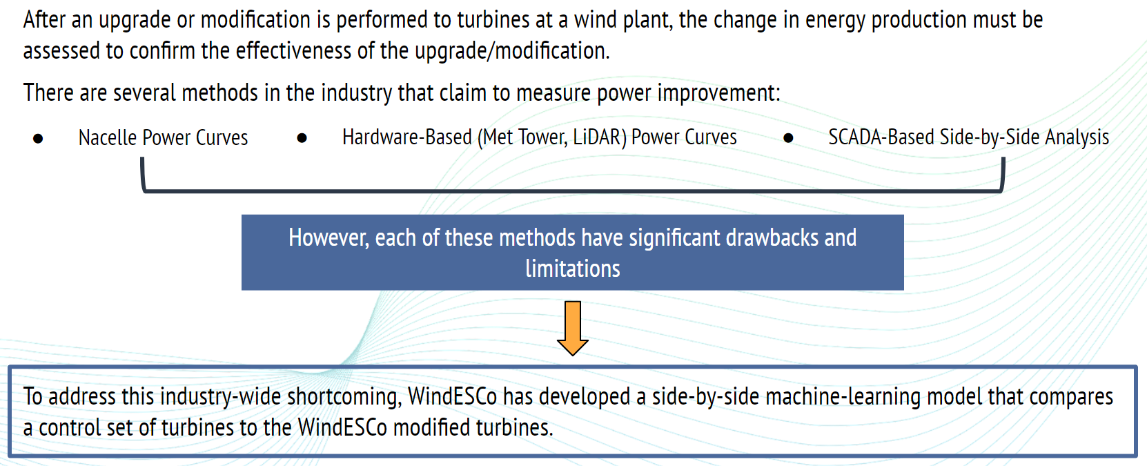
In sum, to address the shortcomings in the common approaches to measuring energy production improvement, WindESCo has developed a variation of the traditional side-by-side analysis, grouping turbines and using machine learning to measure the relative change in performance of one group of Test turbines compared to another group of Control Turbines.
- This approach has undergone multiple improvements (now Version 3.0) and is approved DNV. The DNV review and approval was made considering the best practices in machine learning and international guidelines on the assessment of uncertainty
FAQs:
Do we use wind speed as input in the baseline model?
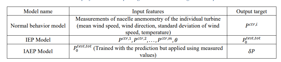
There are three machine learning models used in the EIA - a Normal Behavior model, the IEP model, and the IAEP model. The chart below highlights the inputs and outputs for each of the machine learning models. The baseline or IEP model uses the power of individual control turbines along with a singular wind direction estimate as input features.
What kind of machine learning models are used?
A gradient boosting ML mode (light GBM) l is used. Gradient boosting ML models are chosen because of their capacity in capturing nonlinear behavior in training data. Two other gradient boosting ML models are used to predict the upper and lower quantile ranges (for a 95% CI) for these estimates.
How do we calculate the AEP?
The IEP model is used to predict the power of the test turbine group based on the global wind direction and the control turbine group power. These power forecasts can be compared with the actual power of the test turbine group to define a distribution of power deltas (i.e., predicted test turbine group power minus estimated test turbine group power). This distribution of power deltas is used to train another ML model, the Improvement in Annual Energy Production (IAEP) model, which defines the relationship between the predicted test turbine group and the measured power difference (i.e., the difference attributed to the turbine control change). Once this ML model is trained, the annual power distribution can be passed through the model to quantify the expected improvement in annual energy production due to the turbine control change(s). Effectively, this model is normalizing the difference in power production between the baseline and optimized periods to the annual power distribution.
Does the windiness of the specific year have an impact on the EIA?
Yes, the annual wind conditions (e.g., windiness) could have an impact on the expected improvement in annual energy production. Similarity scores are derived that measure the level of similarity in the wind and atmospheric conditions between the respective training and forecast periods. Sample outputs of these similarity scores, such as the wind profile similarity socre and the IEP feature space score, are provided below.

Comparing the wind and atmospheric conditions between the baseline, optimized, and annual conditions ensure the different ML models are not extrapolating to conditions they were not sufficiently trained on. As an internal metric, WindESCo uses a threshold of 70% to deem whether sufficient training data were available. The similarity scores compare distributions of wind speed, wind direction, ambient temperature, turbine power, and online status.
How can you avoid the problem of overfitting?
Four-fold cross-validation can be used to avoid overfitting; this also helps to ensure the control turbines being used in the ML model were impactful to the learned relationship between the control and test turbine groups.
Can you provide additional insight into how you derive uncertainty?
Information on how uncertainty is derived is defined in the DNV document, WindESCo Energy Improvement Analysis v3.0. A gradient boosting type ML (i.e., light GBM) model is used to predict the expectation of the target, and two additional gradient boost type ML models are trained to predict the lower and upper quantiles of the target (when a 95% confidence level is selected, the lower and upper quantiles are 2.5% and 97.5%). The uncertainty is quantified by subtracting the predicted value from the lower and upper quantiles. Note that the distribution of the prediction uncertainty is not in general symmetric because values derived from the lower and upper quantiles are different. However, to simplify the expression, the uncertainty may be approximated as the half range of the two quantiles.